Getting Started
This section provides an overview on what PyTrajectory is and how to use it. For a more detailed view please have a look at the PyTrajectory Modules Reference.
Contents
What is PyTrajectory?
PyTrajectory is a Python library for the determination of the feed forward control to achieve a transition between desired states of a nonlinear control system.
Planning and designing of trajectories represents an important task in the control of technological processes. Here the problem is attributed on a multi-dimensional boundary value problem with free parameters. In general this problem can not be solved analytically. It is therefore resorted to the method of collocation in order to obtain a numerical approximation.
PyTrajectory allows a flexible implementation of various tasks and enables an easy
implementation. It suffices to supply a function  that represents the
vectorfield of a control system and to specify the desired boundary values.
that represents the
vectorfield of a control system and to specify the desired boundary values.
Installation
PyTrajectory has been developed and tested on Python 2.7
If you have troubles installing PyTrajectory, please don’t hesitate to contact us.
Dependencies
Before you install PyTrajectory make sure you have the following dependencies installed on your system.
- numpy
- sympy
- scipy
- optional
- matplotlib [visualisation]
- ipython [debugging]
PyPI
The easiest way of installing PyTrajectory would be
$ pip install pytrajectory
provided that you have the Python module pip installed on your system.
Source
To install PyTrajectory from the source files please download the latest release from here. After the download is complete open the archive and change directory into the extracted folder. Then all you have to do is run the following command
$ python setup.py install
Please note that there are different versions of PyTrajectory available (development version in github repository [various branches], release versions at PyPI). Because the documentation is build automatically upon the source code, there are also different versions of the docs available. Please make sure that you always use matching versions of code and documentation.
Windows
To install PyTrajectory on Windows machines please make sure you have already installed Python version 2.7 on your system. If not, please download the latest version and install it by double-clicking the installer file.
To be able to run the Python interpreter from any directory we have to append the PATH environment variable. This can be done by right-clicking the machine icon (usually on your Desktop, called My Computer), choosing Properties, selecting Advance and hitting Environment Variables. Then select the PATH (or Path) variable, click Edit an append the following at the end of the line
;C:\Python27\;C:\Python27\Scripts\
If you can’t find a variable called PATH you can create it by clicking New, naming it PATH and insert the line above without the first `;` as the value.
Before going on, open a command line with the shortcut consisting of the Windows-key and the R-key. Run cmd and after the command line interface started type the following:
C:\> pip --version
If it prints the version number of pip you can skip the next two steps. Else, the next thing to do is to install a Python software package called Setuptools that extends packaging and installation facilities. To do so, download the Python script ez_setup.py and run it by typing
C:>\path\to\file\python ez_setup.py
To simplify the installation of new packages we install a software called pip. This is simply done by downloading the file get_pip.py and running
C:>\path\to\file\python get_pip.py
from the command line again.
After that, (and after you have installed the dependencies with a similar command like the next one) you can run
C:>\pip install pytrajectory
and pip should manage to install PyTrajectory.
Again, if you have troubles installing PyTrajectory, please contact us.
Note
The information provided in this section follows the guide available here.
MAC OSX
To install PyTrajectory on machines running OSX you first have to make sure there is Python version 2.7 installed on your system (should be with OSX >= 10.8). To check this, open a terminal and type
$ python --version
If this is not the case we have to install it (obviously). To do so we will use a package manager called Homebrew that allows an installation procedure similar to Linux environments. But before we do this pease check if you have XCode installed.
Homebrew can be installed by opening a terminal and typing
$ ruby -e "$(curl -fsSL https://raw.githubusercontent.com/Homebrew/install/master/install)"
Once Homebrew is installed we insert its directory at the top of the PATH environment variable by adding the following line at the bottom of your ~.profile file (you have to relogin for this to take effect)
export PATH=/usr/local/bin:/usr/local/sbin:$PATH
Now, installing Python version 2.7 is as easy as typing
$ brew install python2
into a terminal. Homebrew also will install packages called Setuptools and pip that manage the installation of additional Python packages.
Now, before installing PyTrajectory please make sure to install its dependencies via
$ pip install sympy
and similar commands for the others. After that you can install Pytrajectory by typing
$ pip install pytrajectory
or install it from the source files.
Again, if you have troubles installing PyTrajectory, please contact us.
Note
The information provided in this section follows the guide available here.
Usage
In order to illustrate the usage of PyTrajectory we consider the following simple example.
A pendulum mass  is connected by a massless rod of length
  to a cart
  on which a force
  acts to accelerate it.
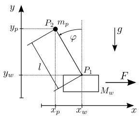
A possible task would be the transfer between two angular positions of the pendulum.
In this case, the pendulum should hang at first down ( ) and is
to be turned upwards (
) and is
to be turned upwards ( ). At the end of the process, the car should be at
the same position and both the pendulum and the cart should be at rest.
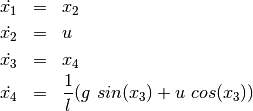
The (partial linearised) system is represented by the following differential equations,
where
). At the end of the process, the car should be at
the same position and both the pendulum and the cart should be at rest.
The (partial linearised) system is represented by the following differential equations,
where ![[x_1, x_2, x_3, x_4] = [x_w, \dot{x_w}, \varphi, \dot{\varphi}]](../_images/math/0ee49f05e559cd6e9155c3ff4ca086ad4efd7665.png) and
and
 is our control variable:
To solve this problem we first have to define a function that returns the vectorfield of
the system above. Therefor it is important that you use SymPy functions if necessary, which is
the case here with  and
and  .
.
So in Python this would be
>>> from sympy import sin, cos
>>>
>>> def f(x,u):
...     x1, x2, x3, x4 = x  # system variables
...     u1, = u             # input variable
...
...     l = 0.5     # length of the pendulum
...     g = 9.81    # gravitational acceleration
...
...     # this is the vectorfield
...     ff = [          x2,
...                     u1,
...                     x4,
...         (1/l)*(g*sin(x3)+u1*cos(x3))]
...
...     return ff
...
>>>
Wanted is now the course for  , which transforms the system with the following start
and end states within
, which transforms the system with the following start
and end states within ![T = 2 [s]](../_images/math/48ac522661f248b225e21d35d8eb668d3cd75a73.png) .
.
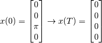
so we have to specify the boundary values at the beginning
>>> from numpy import pi
>>>
>>> a = 0.0
>>> xa = [0.0, 0.0, pi, 0.0]
and end
>>> b = 2.0
>>> xb = [0.0, 0.0, 0.0, 0.0]
The boundary values for the input variable are
>>> ua = [0.0]
>>> ub = [0.0]
because we want  .
.
Now we import all we need from PyTrajectory
>>> from pytrajectory import ControlSystem
and pass our parameters.
>>> S = ControlSystem(f, a, b, xa, xb, ua, ub)
All we have to do now to solve our problem is
>>> x, u = S.solve()
After the iteration has finished x(t) and u(t) are returned as callable functions for the system and input variables, where t has to be in (a,b).
In this example we get a solution that satisfies the default tolerance
for the boundary values of  after the 7th iteration step
with 320 spline parts. But PyTrajectory enables you to improve its
performance by altering some of its method parameters.
after the 7th iteration step
with 320 spline parts. But PyTrajectory enables you to improve its
performance by altering some of its method parameters.
For example if we increase the factor for raising the spline parts (default: 2)
>>> S.set_param('kx', 5)
and don’t take advantage of the system structure (integrator chains)
>>> S.set_param('use_chains', False)
we get a solution after 3 steps with 125 spline parts.
There are more method parameters you can change to speed things up, i.e. the type of collocation points to use or the number of spline parts for the input variables. To do so, just type:
>>> S.set_param('<param>', <value>)
Please have a look at the PyTrajectory Modules Reference for more information.
Visualisation
Beyond the simple plot method (see: PyTrajectory Modules Reference)
PyTrajectory offers basic capabilities to animate the given system.
This is done via the Animation class from the utilities
module. To explain this feature we take a look at the example above.
When instanciated, the Animation requires the calculated
simulation results T.sim and a callable function that draws an image
of the system according to given simulation data.
First we import what we need by:
>>> import matplotlib as mpl
>>> from pytrajectory.visualisation import Animation
Then we define our function that takes simulation data x of a specific time and an instance image of Animation.Image which is just a container for the image. In the considered example xt is of the form
![\begin{equation*}
xt = [x_1, x_2, x_3, x_4] = [x_w, \dot{x}_w, \varphi, \dot{\varphi}]
\end{equation*}](../_images/math/856f63b13ff9fe0aff52c702bc739df5eeaeab3b.png)
and image is just a container for the drawn image.
def draw(xt, image):
    # to draw the image we just need the translation `x` of the
    # cart and the deflection angle `phi` of the pendulum.
    x = xt[0]
    phi = xt[2]

    # next we set some parameters
    car_width = 0.05
    car_heigth = 0.02

    rod_length = 0.5
    pendulum_size = 0.015

    # then we determine the current state of the system
    # according to the given simulation data
    x_car = x
    y_car = 0

    x_pendulum = -rod_length * sin(phi) + x_car
    y_pendulum = rod_length * cos(phi)

    # now we can build the image

    # the pendulum will be represented by a black circle with
    # center: (x_pendulum, y_pendulum) and radius `pendulum_size
    pendulum = mpl.patches.Circle(xy=(x_pendulum, y_pendulum), radius=pendulum_size, color='black')

    # the cart will be represented by a grey rectangle with
    # lower left: (x_car - 0.5 * car_width, y_car - car_heigth)
    # width: car_width
    # height: car_height
    car = mpl.patches.Rectangle((x_car-0.5*car_width, y_car-car_heigth), car_width, car_heigth,
                                fill=True, facecolor='grey', linewidth=2.0)

    # the joint will also be a black circle with
    # center: (x_car, 0)
    # radius: 0.005
    joint = mpl.patches.Circle((x_car,0), 0.005, color='black')

    # and the pendulum rod will just by a line connecting the cart and the pendulum
    rod = mpl.lines.Line2D([x_car,x_pendulum], [y_car,y_pendulum],
                            color='black', zorder=1, linewidth=2.0)

    # finally we add the patches and line to the image
    image.patches.append(pendulum)
    image.patches.append(car)
    image.patches.append(joint)
    image.lines.append(rod)

    # and return the image
    return image
If we want to save the latest simulation result, maybe because the iteration took much time and we don’t want to run it again every time, we can do this.
S.save(fname='ex0_InvertedPendulumSwingUp.pcl')
Next, we create an instance of the Animation class and
pass our draw function, the simulation data and some
lists that specify what trajectory curves to plot along with the
picture.
If we would like to either plot the system state at the end time or want to animate the system we need to create an Animation object. To set the limits correctly we calculate the minimum and maximum value of the cart’s movement along the x-axis.
    A = Animation(drawfnc=draw, simdata=S.sim_data,
                  plotsys=[(0,'x'), (2,'phi')], plotinputs=[(0,'u')])

    # as for now we have to explicitly set the limits of the figure
    # (may involves some trial and error)
    xmin = np.min(S.sim_data[1][:,0]); xmax = np.max(S.sim_data[1][:,0])
    A.set_limits(xlim=(xmin - 0.5, xmax + 0.5), ylim=(-0.6,0.6))
Finally, we can plot the system and/or start the animation.
if 'plot' in sys.argv:
    A.show(t=S.b)

if 'animate' in sys.argv:
    # if everything is set, we can start the animation
    # (might take some while)
    A.animate()
The animation can be saved either as animated .gif file or as a .mp4 video file.
A.save('ex0_InvertedPendulum.gif')
If saved as an animated .gif file you can view single frames using for example gifview (GNU/Linux) or the standard Preview app (OSX).