Non-Standard Approach¶

There are implemented two different approaches for the polynomial parts of the splines in PyTrajectory. They differ in the choice of the nodes. Given an interval $[x_k, x_{k+1}],\ k \in [0, \ldots, N-1]$ the standard way in spline interpolation is to define the corresponding polynomial part using the left endpoint by

$P_k(t) = c_{k,0} (t - x_k)^3 + c_{k,1}(t - x_k)^2 + c_{k,2}(t - x_k) + c_{k,3}$

However, in the thesis of O. Schnabel from which PyTrajectory emerged a different approach is used. He defined the polynomial parts using the right endpoint, i.e.

$P_k(t) = c_{k,0} (t - x_{k+1})^3 + c_{k,1}(t - x_{k+1})^2 + c_{k,2}(t - x_{k+1}) + c_{k,3}$

This results in a different matrix to ensure the smoothness and boundary conditions of the splines:

$\setcounter{MaxMatrixCols}{20} \setlength{\arraycolsep}{3pt} \newcommand\bigzero{\makebox(0,0){\text{\huge0}}} \begin{equation*} \textstyle \underbrace{\begin{bmatrix} 0 & 0 & 0 & 1 & h^3 & -h^2 & h & -1 \\ 0 & 0 & 1 & 0 & -3h^2 & 2h & -1 & 0 &&&& \bigzero \\ 0 & 2 & 0 & 0 & 6h & -2 & 0 & 0 \\ & & & & 0 & 0 & 0 & 1 & h^3 & -h^2 & h & -1 \\ & \bigzero & & & 0 & 0 & 1 & 0 & -3h^2 & 2h & -1 & 0 &&&&&& \bigzero \\ & & & & 0 & 2 & 0 & 0 & 6h & -2 & 0 & 0 \\ &&&&&&&&&&& \ddots \\ & & & & & & & & & & & & 0 & 0 & 0 & 1 & h^3 & -h^2 & h & -1 \\ & & & & & & \bigzero & & & & & & 0 & 0 & 1 & 0 & -3h^2 & 2h & -1 & 0 \\ & & & & & & & & & & & & 0 & 2 & 0 & 0 & 6h & -2 & 0 & 0 \\ & & & & & & & & & & & & & \\ -h^3 & h^2 & -h & 1 \\ 3h^2 & -2h & 1 & 0 &&&&&&&& \bigzero \\ -6h & 2 & 0 & 0 \\ & & & & & & & & & & & & & & & & 0 & 0 & 0 & 1 \\ & & & & & & \bigzero & & & & & & & & & & 0 & 0 & 1 & 0 \\ & & & & & & & & & & & & & & & & 0 & 2 & 0 & 0 \\ \end{bmatrix}}_{=: \boldsymbol{M}} \end{equation*}$

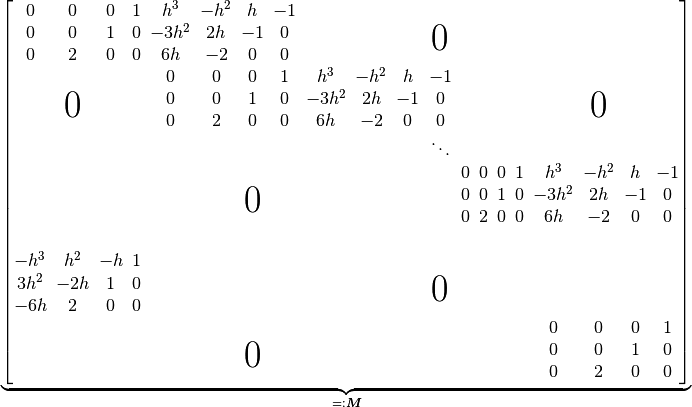
The reason for the two different approaches being implemented is that after implementing and switching to the standard approach some of the examples no longer converged to a solution. The examples that are affected by that are: