Acrobot¶

One further interesting example is that of the acrobot. The model can be regarded as a simplified gymnast hanging on a horizontal bar with both hands. The movements of the entire system is to be controlled only by movement of the hip. The body of the gymnast is represented by two rods which are jointed in the joint $G_2$ . The first rod is movably connected at joint $G_1$ with the inertial system, which corresponds to the encompassing of the stretching rod with the hands.

For the model, two equal-length rods with a length $l_1 = l_2 = l$ are assumed with a homogeneous distribution of mass $m_1 = m_2 = m$ over the entire rod length. This does not correspond to the proportions of a man, also no restrictions were placed on the mobility of the hip joint.

The following figure shows the schematic representation of the model.

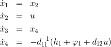
Using the previously assumed model parameters and the write abbreviations

$\begin{eqnarray*} I & = & \frac{1}{3}m l^2 \\ d_{11} & = & \frac{m l^2}{4} + m(l^2 + \frac{l^2}{4} + l^2 \cos(\theta_2)) + 2I \\ h_1 & = & - \frac{m l^2}{2} \sin(\theta_2) (\dot{\theta}_2 (\dot{\theta}_2 + 2\dot{\theta}_1)) \\ d_{12} & = & m (\frac{l^2}{4} + \frac{l^2}{2} \cos(\theta_1)) + I \\ \varphi_1 & = & \frac{3}{2}m l g \cos(\theta_1) + \frac{1}{2}m l g \cos(\theta_1 + \theta_2) \end{eqnarray*}$

as well as the state vector $x = [\theta_2, \dot{\theta}_2, \theta_1, \dot{\theta}_1]$ one obtains the following state representation with the virtual input $u = \ddot{\theta}_2$

$\begin{eqnarray*} \dot{x}_1 & = & x_2 \\ \dot{x}_2 & = & u \\ \dot{x}_3 & = & x_4 \\ \dot{x}_4 & = & -d_{11}^{-1} (h_1 + \varphi_1 + d_{12}u) \end{eqnarray*}$

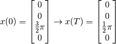
Now, the trajectory of the manipulated variable for an oscillation of the gymnast should be determined. The starting point of the exercise are the two downward hanging rods. These are to be transferred into another rest position in which the two bars show vertically upward within an operating time of $T = 2 [s]$ . At the beginning and end of the process, the input variable is to merge continuously into the rest position $u(0) = u(T) = 0$ .

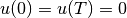The initial and final states thus are

$\begin{equation*} x(0) = \begin{bmatrix} 0 \\ 0 \\ \frac{3}{2} \pi \\ 0 \end{bmatrix} \rightarrow x(T) = \begin{bmatrix} 0 \\ 0 \\ \frac{1}{2} \pi \\ 0 \end{bmatrix} \end{equation*}$

Source Code¶# acrobot

# import trajectory class and necessary dependencies
from pytrajectory import ControlSystem
import numpy as np
from sympy import cos, sin

# define the function that returns the vectorfield
def f(x,u):
    x1, x2, x3, x4 = x
    u1, = u
    
    m = 1.0             # masses of the rods [m1 = m2 = m]
    l = 0.5             # lengths of the rods [l1 = l2 = l]
    
    I = 1/3.0*m*l**2    # moments of inertia [I1 = I2 = I]
    g = 9.81            # gravitational acceleration
    
    lc = l/2.0
    
    d11 = m*lc**2+m*(l**2+lc**2+2*l*lc*cos(x1))+2*I
    h1 = -m*l*lc*sin(x1)*(x2*(x2+2*x4))
    d12 = m*(lc**2+l*lc*cos(x1))+I
    phi1 = (m*lc+m*l)*g*cos(x3)+m*lc*g*cos(x1+x3)

    ff = np.array([     x2,
                        u1,
                        x4,
                -1/d11*(h1+phi1+d12*u1)
                ])
    
    return ff


# system state boundary values for a = 0.0 [s] and b = 2.0 [s]
xa = [  0.0,
        0.0,
        3/2.0*np.pi,
        0.0]

xb = [  0.0,
        0.0,
        1/2.0*np.pi,
        0.0]

# boundary values for the inputs
ua = [0.0]
ub = [0.0]

# create System
first_guess = {'seed' : 1529} # choose a seed which leads to quick convergence
S = ControlSystem(f, a=0.0, b=2.0, xa=xa, xb=xb, ua=ua, ub=ub, use_chains=True, first_guess=first_guess)

# alter some method parameters to increase performance
S.set_param('su', 10)

# run iteration
S.solve()