Underactuated Manipulator¶

In this section, the model of an underactuated manipulator is treated. The system consists of two bars with the mass $M_1$ and $M_2$ which are connected to each other via the joint $G_2$ . The angle between them is designated by $\theta_2$ . The joint $G_1$ connects the first rod with the inertial system, the angle to the $x$ -axis is labeled $\theta_1$ . In the joint $G_1$ the actuating torque $Q$ is applied. The bars have the moments of inertia $I_1$ and $I_2$ . The distances between the centers of mass to the joints are $r_1$ and $r_2$ .

The modeling was taken from the thesis of Carsten Knoll (April, 2009) where in addition the inertia parameter $\eta$ was introduced.

$\begin{equation*} \eta = \frac{m_2 l_1 r_2}{I_2 + m_2 r_2^2} \end{equation*}$

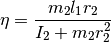
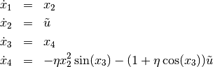
For the example shown here, strong inertia coupling was assumed with $\eta = 0.9$ . By partial linearization to the output $y = \theta_1$ one obtains the state representation with the states $x = [\theta_1, \dot{\theta}_1, \theta_2, \dot{\theta}_2]^T$ and the new input $\tilde{u} = \ddot{\theta}_1$ .

$\begin{eqnarray*} \dot{x}_1 & = & x_2 \\ \dot{x}_2 & = & \tilde{u} \\ \dot{x}_3 & = & x_4 \\ \dot{x}_4 & = & -\eta x_2^2 \sin(x_3) - (1 + \eta \cos(x_3))\tilde{u} \end{eqnarray*}$

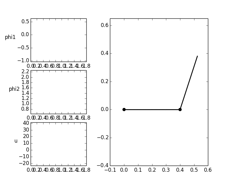
For the system, a trajectory is to be determined for the transfer between two equilibrium positions within an operating time of $T = 1.8 [s]$ .

$\begin{equation*} x(0) = \begin{bmatrix} 0 \\ 0 \\ 0.4 \pi \\ 0 \end{bmatrix} \rightarrow x(T) = \begin{bmatrix} 0.2 \pi \\ 0 \\ 0.2 \pi \\ 0 \end{bmatrix} \end{equation*}$

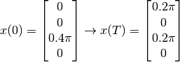
The trajectory of the inputs should be without cracks in the transition to the equilibrium positions (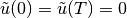 $\tilde{u}(0) = \tilde{u}(T) = 0$ ).

Source Code¶# underactuated manipulator

# import trajectory class and necessary dependencies
from pytrajectory import ControlSystem
import numpy as np
from sympy import cos, sin

# define the function that returns the vectorfield
def f(x,u):
    x1, x2, x3, x4  = x     # state variables
    u1, = u                 # input variable
    
    e = 0.9     # inertia coupling
    
    s = sin(x3)
    c = cos(x3)
    
    ff = np.array([         x2,
                            u1,
                            x4,
                    -e*x2**2*s-(1+e*c)*u1
                    ])
    
    return ff

# system state boundary values for a = 0.0 [s] and b = 1.8 [s]
xa = [  0.0,
        0.0,
        0.4*np.pi,
        0.0]

xb = [  0.2*np.pi,
        0.0,
        0.2*np.pi,
        0.0]

# boundary values for the inputs
ua = [0.0]
ub = [0.0]

# create trajectory object
S = ControlSystem(f, a=0.0, b=1.8, xa=xa, xb=xb, ua=ua, ub=ub)

# also alter some method parameters to increase performance
S.set_param('su', 20)
S.set_param('kx', 3)

# run iteration
S.solve()