Swing up of the inverted dual pendulum
In this example we add another pendulum to the cart in the system.
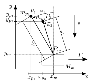
The system has the state vector ![x = [x_1, \dot{x}_1,
\varphi_1, \dot{\varphi}_1, \varphi_2, \dot{\varphi}_2]](../../_images/math/c3523c6297f81560dfe6b7a6d779273f1d9074dd.png) . A partial
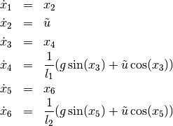
linearization with
. A partial
linearization with  yields the following system state
representation where
yields the following system state
representation where  .
.
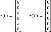
Here a trajectory should be planned that transfers the system between
the following two positions of rest. At the beginning both pendulums
should be directed downwards ( ).
After a operating time of
).
After a operating time of ![T = 2 [s]](../../_images/math/48ac522661f248b225e21d35d8eb668d3cd75a73.png) the cart should be at the
same position again and the pendulums should be at rest with
the cart should be at the
same position again and the pendulums should be at rest with
 .
.
Source Code
# swing up of the inverted dual pendulum with partial linearization

# import trajectory class and necessary dependencies
from pytrajectory import ControlSystem
from sympy import cos, sin
import numpy as np

# define the function that returns the vectorfield
def f(x,u):
    x1, x2, x3, x4, x5, x6 = x  # system variables
    u, = u                      # input variable

    # length of the pendulums
    l1 = 0.7
    l2 = 0.5

    g = 9.81    # gravitational acceleration

    ff = np.array([         x2,
                            u,
                            x4,
                (1/l1)*(g*sin(x3)+u*cos(x3)),
                            x6,
                (1/l2)*(g*sin(x5)+u*cos(x5))
                    ])

    return ff

# system state boundary values for a = 0.0 [s] and b = 2.0 [s]
xa = [0.0, 0.0,  np.pi, 0.0,  np.pi, 0.0]
xb = [0.0, 0.0, 0.0, 0.0, 0.0, 0.0]

# boundary values for the input
ua = [0.0]
ub = [0.0]

# create trajectory object
S = ControlSystem(f, a=0.0, b=2.0, xa=xa, xb=xb, ua=ua, ub=ub)

# alter some method parameters to increase performance
S.set_param('su', 10)
S.set_param('eps', 8e-2)

# run iteration
S.solve()